

This project is part of a bigger plan to implement a more complex water simulation material, utilizing FFT based wave generation (as seen in Tessendorf’s Simulating Ocean Water).
In its current form it uses Fractional Brownian Motion to generate a variable number of wave signals that get summed together to compute the final displacement of the mesh.
The material then uses the function derivative to compute the normal. The height function is also used to compute tessellation, this material can thus be used with a simple quad. All parameters can be modified from the user’s side and there is also an option for choosing different functions as the kernel of the sum (e.g.).
You can read more about it here and you can find the source code on my github here. The final material currently uses basic Blinn Phong as it allows for easier visual debugging compared to a PBR model, which will be implemented together with the FFT version of the material.
The Maths of Water Generation
Being able to replicate natural phenomena via precise and efficient mathematical models is definitely one of the most interesting problems tackled in the space of simulation, both real time (e.g. Video Games) and offline (e.g. Automotive). The problem of generating a realistic looking body of water has thus been something game developers have been tackling for many years, since utilizing actual fluid simulation is unfeasible when you have a render budget of 16ms in which you have to fit the entire computation plus whatever else you are doing that depends on it. This project was the perfect chance to explore how the maths evolved from the very first (and very well known) published water simulation algorithm for real time use cases to today’s FFT based algorithms used both in Cinema and Video Games which can support more complex behaviors such as foreign body generated wakes and foam formation (scientifically known as whitecap).
Fundamentals
A lot of the things covered here will use a mix of calculus and trigonometry, so it’s useful to refresh the things that are going to be needed for the rest of the formulas that will be shown. If you’re familiar with these topics this is a very skippable section.
Sine, Cosine and the Unit Circle
We very often use sine and cosine functions in shaders to be able to pass from a linear set of values to a periodic one (in , both and will yield the same result) but how are they actually defined?
For this we need to take the unit circle, that is a circle in the cartesian plane whose radius is equal to one.

You can mathematically describe this circle by utilising Pythagoras’ Theorem and have that: .
You’ll have that you’ll be able to solve this equation only for values of x and y that place a point on the red line. Thus at any given angle between the x axis and an arbitrary line going through the center, there will be a corresponding pair of x and y values that will place a point on the unit circle. That’s where sine and cosine come in, where they are the function that returns, respectively, the y coordinate and the x coordinate of the point for any given angle.
Derivatives and Partial Derivatives
Derivatives are a foundational block to be able to go from a function that only computes displacement of a mesh to computing the normal vector at any point on the mesh, thus unlocking the possibility to shade a quad with much more detail beyond the one available to us at a vertex level. Derivatives inform us on the difference between two points in a function. If you take any two points and for the function , the change between the two points is defined as:
The derivative is what we get when we try to get two points infinitesimally close together.
For a constant value this would be 0, because whatever point you choose its value is always the same, for a linear function of the type it would be , since the constant value yields a 0 change over two points while is the slope with which the values of the function change. Here is a quick recap of useful derivatives.
Partial derivatives are instead derivatives when it comes to multiple dimensions. Since the derivatives inform us about the rate of change of a function in only one dimension, partial derivatives allow us to isolate one dimension at a time. They can be computed by assuming all other dimensions remain constant (it’s as if you’re taking a very small slice of the function where this is true)
e.g. with , I won’t be rigorous and use to indicate that component is fully constant for that dimension.
First Waves : Sum of Sines
Let’s start by trying to model wave behavior in just one dimension. The most simple way to imagine water body motion is to imagine forces such as foreign body moving in it, wind and collision with objects slightly compressing the water around them. Each one generates a wave that gets stacked on top of the others. This approach to generating a water like effect is the one of stacking together different wave functions, for example sine waves. Take the case of the following function sum, where represents time:
While it still does not convey a natural water looking behaviour, you can definitely notice how it is going in the right direction, compared to one single sine wave, which instead looks very abstract.

To generalize the formulation let’s take and from an array of values and respectively modify the amplitude, frequency and phase of the wave function.
So now we can choose a set of parameters for the three arrays such that we generate a close enough looking function to water body behavior. It is userful here to observe how the derivatives behave.
Since this is a sum of functions, we can easily compute at any point the line tangent to the function via its derivative. Given that and that We have that :
This is going to be extremely useful later, in the 3D evolution of this, as it allows us to also compute the line normal to the function at any point, given it’s just the line perpendicular to the tangent one .
N.B. Knowing the slope of a function, we can get vectors along the line as either or , in our case we are going to set as the wave normals never point down in any fashion.

Moreover, because of energy conservation, bigger amplitude waves will need to have lower frequency values and viceversa. This is also true for real water as we don’t really see very high waves with a high frequency, but rather small frequent ripples together with bigger waves with a lower frequency.
Reigning in Complexity: Fractional Brownian Motion
Being able to select a full list of values for the wave function definitely opens up a big space for customization of the look of the final wave, but authoring 10+ parameters and fine tuning them definitely becomes overwhelming quickly, but we still need enough waves to get good detail. We can take into consideration energy conservation from before to leverage a mathematical concept to add constraints on the way we generate the waves, without forgoing the ability to modify the final look.
Fractional Brownian Motion is the generalization of Brownian Motion, which, in few words, is the concept of a sequence of random values, where each one is not correlated to the next one. In the case of FBM, instead, we do allow for some correlation, as we will be seeing now.
If we redefine in the following way, we can much more easily scale the number of waves without having to handle parameters each time.
So we ultimately define a sum of wave functions where at each step, starting from the base values of for ampltidue, frequency and phase:
- The amplitude decreases by a factor of
- The phase and the frequency increase by a factor of and
We will call the factors ramps from now on, as they ultimately describe how steep the values ramp down or up.
So ultimately now we have at any point a pseudo random number where each value still correlates with the others, given the parameters are all computed from the same starting values. The full mathematical definition of FBM is more complex and precise while in our case it indicates just the emulation of random behavior by layering multiple functions together with constants that are correlated across each layer.
So now from having parameters for our function, we only have 6 (starting + ramp) and they still allow for a good amount of customization.
Here is a quick hlsl snippet summarizing the current wave generation process. And here is an example shader showing the result of the sum of sines with 32 iterations. The colour of the line also describes the slope of the normal line over the length of the wave.
#define WaveFunc sin#define WaveFuncDerivative cos#define WAVE_NUM 32
float GetWaveHeight(float x, float time, float A, float W, float P, float amplitudeRamp, float frequencyRamp, float phaseRamp){ float h = 0; for (int i=0; i< WAVE_NUM; i++){ h += A * pow(amplitudeRamp, i) * WaveFunc( W * pow(frequencyRamp,i) * x + P * pow(phaseRamp, i) * time); } return h;}
float GetWaveNormalLine(float x, float time, float A, float W, float P, float amplitudeRamp, float frequencyRamp, float phaseRamp){ float m = 0; for (int i=0; i< WAVE_NUM; i++){ m += A * pow(amplitudeRamp, i) * W * pow(frequencyRamp,i) * WaveFuncDerivative( W * pow(frequencyRamp,i) * x + P * pow(phaseRamp, i) * time); } // This is the slope of the line normal to the function, // described as y = (-1/m)*x. If we wanted the direction // of the normal vector we could just get it as float2(-m, 1) return -1/m;}Addressing Wave Peaks
One other thing missing from the wave function in order to give it a more natural look is peaks. Beyond actual breaking waves (which are much more complex phenomenon that are closer to the realm of full fluid simulation), peaks are one of the characteristic features of waves. In order to have this, instead of playing around with the way we generate the parameters such as amplitude, phase etc… we can change the actual kernel of the sum. We are currently using the sine function, but we do have options that have a more peaky appearance: Gerstner Waves and Exponential Sines. This will change our functions a bit.
Gerstner Waves operate a bit differently, utilizing the input value to generate both coordinates in the x and y dimension, the function for the y dimension stays the same, utilizing as input of the sine function, while x becomes the following, wehre is another factor accounting for the steepness of the wave:
Here is the new functions when using the exponential sine instead:
For simplicity I’ll focus on the exponential sine, as Gerstner Waves are notoriously prone to easily breaking when parameters go out of range, thus needing more specific curation. Here is the same shader as before, but utilizing the exponential sine as kernel function instead.
Going 3D
Up until now we have seen all the foundational math to essentially generate a wave signal that allows us to reproduce wave behavior in two dimensions, but once understood this, expanding to the three-dimensional case is a matter of essentially adding one more wave signal and taking into account the bidemnsional nature of the wave direction.
Directing the waves
In two dimensions, the waves can go into one of two directions: right or left, but this behavior scales quickly when going 3D, as now the direction of a wave can be any of the 360 degrees over the surface of the horizontal plane.

The way we can model this behavior is simpler than it looks. Looking at it from the top, you can imagine the sine wave as a function that will give values to based on some contribution from the and variables. We thus define factors which represent the contribution of and to the sine function computing . We also see that and can describe a vector that represents the direction of the wave, rewriting in a shorter form.
Let’s also rewrite this in a -up system, given the final HLSL code will be written for Unity, which uses a -up, left handed coordinate system. We also rewrite the derivative for each dimension, which we will need to compute the partial derivatives of the function.
This applies to any of the previous kernel functions, so now we can rewrite the previous 2D FBM algorithm in its three dimensional form, keeping in mind that we are going to randomize for each iteration of the FBM, yielding a different at each step. This will allow us to sum together wave signals developing in different directions, replicating the effect of waves being generated from different sources (wind, previous waves bouncing off the shore etc…)
Computing the normal
In the 2D case of wave generation we were able to obtain the line that is normal to any point of the function by first computing the slope of the tangent line (i.e. the derivative of the function at the point) and then finding the line perpendicular to it. We’ll operate similarly to find the normal vector at any point, starting from the partial derivatives over the two horizontal directions . With the derivatives we’ll compute the two vectors , respectively the vector tangent and binormal of the displaced surface. Given the sine wave now develops over two dimensions, we’ll need two lines tangent to the function, instead of one.
The best way to visualize what is being done is to have a dividi et impera approach. We take a slice of the space so thin over the x and z axis,that the other variable will practically be constant and we can go back to considering the function a 2D function. (Thin slice over x for the z derivative, the opposize for the x derivative). We then compute the derivative for that faux 2D function, thus getting a vector that is necessarily tangent to it. Since the two vectors lie on perpendicular planes ( on plane, on the plane), they are also perpendicular to each other.


From here, getting the normal vector is just a matter of computing the cross product between and , as it’s by definition perpendicular to both.
Note on the math
Here we are using a left-handed coordinate system since we are making the computation in Unity's system. We are also inverting the vector at the end, since we need the vector that is pointing up, same as in the 2D case. It won't affect the computation as it's just a quirk of how we computed the derivatives in that coordinate system.So we now have:
- A wave-line signal we can use to displace a vertex along the vertical axis.
- A derivative of the signal in both horizontal dimensions, allowing us to compute the normal to the surface at any point.
Here is an hlsl snippet summarizing what we can compute so far.
#define WaveFunc ExpSine#define WaveFuncDerivative ExpSineDer#define WAVE_NUM 32
float ExpSine(float x){ return exp(sin(x)-1.0);}float ExpSineDer(float x){ return exp(sin(x)-1.0) * cos(x);}
float Get3DWaveHeight(float x, float z, float2 waveDir, float time, float A, float W, float P, float amplitudeRamp, float frequencyRamp, float phaseRamp){ float h = 0; for (int i=0; i< WAVE_NUM; i++){ h += A * pow(amplitudeRamp, i) * WaveFunc( W * pow(frequencyRamp,i) * (waveDir.x * x + waveDir.y * z) + P * pow(phaseRamp, i) * time); } return h;}
float Get3DWaveNormal(float x, float z, float2 waveDir, float time, float A, float W, float P, float amplitudeRamp, float frequencyRamp, float phaseRamp){ float mx = 0; float mz = 0; for (int i=0; i< WAVE_NUM; i++){ mx += A * pow(amplitudeRamp, i) * W * pow(frequencyRamp,i) * waveDir.x * WaveFuncDerivative( W * pow(frequencyRamp,i) * (waveDir.x * x + waveDir.y * z) + P * pow(phaseRamp, i) * time); mz += A * pow(amplitudeRamp, i) * W * pow(frequencyRamp,i) * waveDir.z * WaveFuncDerivative( W * pow(frequencyRamp,i) * (waveDir.x * x + waveDir.y * z) + P * pow(phaseRamp, i) * time); }
return normalize(-mx,1,-mz);}The Graphics of Water Generation
Now that we have all the mathematical components for our waves, it is time to leverage them in order to get a good looking water material. Starting from applying a lighting model such as Blinn-Phong or PBR, we do have to keep in mind some characteristics of the material to give the water a look closer to ground truth.
Transparency and Reflection
Water behaves in a very specific way when it comes to bouncing off light. Its behaviour can best be seen when looking at a body of water from a shallow angle.
This is a phenomenon shared by all objects, but most visibly translucent and smooth ones (e.g. glass does this as well). It is described by the Fresnel equations. When the light ray hits the surface with an angle smaller than a certain amount, the light gets bounced off the surface entirely instead of crossing the surface. This effect in graphics takes the same name of the equations, and we do have different models for it, one of these is Schlick’s Approximation, which takes the normal vector of the surface, the vector from the point on the surface to the camera, and uses them to compute the final Fresnel factor in the following way.
In this way, when we are looking at a surface straight down (parallel to normal), there will be no Fresnel effect and the object (in our case water) will appear transparent, otherwise it will bounce off light. The body still absors some of the light in any case, so both reflection and refraction will be tinted. We will utilize to determine the strength of the reflection.
- At shallow angles F will be closer to 1, adding a strong reflected color.
- At high angles with the surface, we’ll instead just see through the water.
Starting from the reflected colour, the simplest approach we can have is to compute what colour would be reflected to the observer’s eye. In a simple environment with just one directional light and ambient light we are going to have the following cases:
- If the reflection of the view vector off the surface is parallel (or has a shallow angle) with the directional light, we should bounce off the colour of the directional light itself.
- Otherwise bounce the ambient light.
We can compute the reflected vector simply by taking once again the view vector and the normal vector at the point of the surface . Assuming the view direction doesn’t come from below the surface point, we compute the reflection as
.
We then compute the dot product of the light vector and reflection which will yield the cosine of the angle between the two ( in the picture): it will be close to when the two vectors are almost parallel and pointing in the same hemisphere, 0 when they are perpendicular, when they are parallel but pointing towards opposite hemispheres.

Given we are trying to replicate the ocean and not the shore here, instead of having the surface become transparent we will instead utilise the diffuse colour, replicating the colour coming from the depth of the ocean when we look straight at it. Here is an HLSL snippet summarizing the process.
float3 GetReflectedColor( float3 R, float3 L, float3 lightCol, float sunSize,float lightFalloff, float3 ambientCol){ // We will add a falloff and sun size parameter to doctor how much the sun will be reflected at low angles. This emulates very basicly and approximately the way the atmosphere diffuses the colour of the sun and the fact that the sun is not a point light but rather a three dimensional body emitting light. float reflAngle = dot(R,L); reflAngle = step(1-sunSize, reflAngle); // At 1 the sun will fully encompass the sky, at 0 it will be a point. float d = pow(clamp(reflAngle,0,1), lightFalloff); // The bigger the falloff the less of an "halo" the sun gets. return lerp(ambientCol, lightCol);}
// cameraPos and surfacePoint should be in world space, same as Nfloat3 FinalColor( float3 cameraPos, float3 surfacePoint, float3 N, float3 seaColor, float3 lightColor, float3 ambientColor, float3 L, float sunSize, float lightFalloff){ float3 V = normalize(cameraPos - surfacePoint); float3 R = reflect(V,N); float3 reflectionColor = GetReflectedColor(R,L, lightColor, sunSize, lightFalloff, ambientColor); float fresnelAmt = pow(1-dot(N,V), 5); reflectionColor *= fresnelAmt; float3 diffuse = seaColor; return diffuse + reflectionColor;}Cubemap Reflections
Utilising simply the ambient colour when not reflecting the sun doesn’t actually give off the greatest visual effect, as in reality you rarely have a completely solid colour being reflected, due to atmospherical effects, clouds in the sky, objects in view etc… A cubemap greatly improves the visual quality of reflections in general, and here it is no exception. We already have the vector used to sample it in the reflected vector , so it will just be a matter of using the sampled cubemap as reflected colour.
float3 FinalColor( ... float3 ambientColor samplerCUBE cubeMap ...){ ... float3 R = reflect(V,N); float3 ambientColor = texCUBE(cubeMap, R); ...;}Foam
One other characteristic of sea waves is foam, which is created due to areas of high turbulence. Our mathematical model does not really allow us to know where foam would be present, since it isn’t physically accurate we won’t know where high turbulence is present. What allows us to get something close to it is to look at where it usually forms and trying to emulate it. Foam usually forms around when higher speed areas of the body of water collide, thus generating higher peaks that break into foam. We can use this information to try and compute something out of what makes a peak and what makes a high peak especially. We will thus look at the computed normal from before and compare it against the upward vector as well as use the final value from our displacement function compared against the maximum theoretical value for it.
 A higher point with bigger normal angle (H1,N1) should have more foam compared to a low point that is flatter (H2,N2)
After some fiddling and trial and error, I came out with a simple formula to compute the foam amount with some added parameters to give some authoring capabilities. Starting from the height, given we know the formula to compute the height, we can expect the value for any given iteration step to oscillate between and . This means that we can simply compute the maximum height as the total sum of all the amplitudes.
Note: The amplitude follows a geometric series
We could also leverage the fact that and to compute it all in one line, leveraging the propriety of a geometric series, but the change won't affect the performance that much and adding this to the text would make this more verbose than it already is.So now we have the height of the wave as the ratio between its height and theoretical maximum as well as the angle of the wave at each point with the upward vector as a range . Also, given that foam is a turbulent phenomenon, we do also see that when there is foam the light isn’t reflected at all, so the presence of foam should override any reflection computation. With some trial and error here is the formula I ended up using for the faux foam.
// foamRange, heightFoamAmt, heightFoamFalloff, angleFoamAmt and angleFoamFalloff are all parameters for doctoring the computation here and there. This is far from perfectfloat GetFoamLerp(float h, float maxH, float2 foamRange, float heightFoamAmt, float heightFoamFalloff, float3 n,float angleFoamAmt,float angleFoamFalloff){ float hRatio =saturate(h/maxH); hRatio = (hRatio-foamRange.x)/(foamRange.y-foamRange.x); hRatio = saturate((hRatio - 1 + heightFoamAmt) / heightFoamAmt); hRatio = pow(hRatio, heightFoamFalloff); float angleFoam = DotClamped(float3(0,1,0), n); // Same as doing clamp(normalize(n).y,0,1) angleFoam = saturate((angleFoam -1 + angleFoamAmt) / angleFoamAmt); return lerp(hRatio,pow(angleFoam, angleFoamFalloff), hRatio);}
float3 FinalColor(..., float2 foamReflectionReduction /*another authoring parameter*/){ ... float3 foamL = GetFoamLerp(...); float3 diffuse = lerp(seaColor, foamColor, foamL); reflectionColor = reflectionColor * (1-clamp(foamL, foamReflectionReduction.x,foamReflectionReduction.y)); ...}We now have everything we need:
- A displacement function to move each vertex
- A derivative function to compute the normal vector, thus accurate illumination on a per-fragment basis
- A way to choose between foam and water to better replicate the behavior of the sea
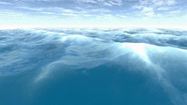
- Parameters that can be changed manually to author the material further. By putting it all together, we can finally get something like the following.
Tessellation
But wait, there is more! We can still leverage the displacement function in another way. Currently the displacement of vertices is bound by the amount of vertices present in the initial mesh. Which can cause the need for quite a bit of vertices if we want to have an accurate represenation of the wave signal we are using.
So we’re going to utilise tessellation to improve the vertex count, only increasing the number of vertices when needed. While standard edge and distance based approaches can offer a working result, they would be limited by the configuration of the starting geometry, given they would lack information regarding the wave signal. An example of such limitation would be the case where two vertices of a tri both would yield a displacement of 0 (thus having the minimum edge distance) while in between them lies the peak of a wave, this would flatten the wave completely. We can improve upon this by leveraging the wave signal itself as the base for the tessellation parameters.
Improving Tessellation with Signal Processing
Let’s start from the observation that there is a threshold (given by the amplitude of each fbm step) below which any new added wave won’t displace the surface enough to require higher vertex density. This will depend on some factors such as the starting amplitude and the ramp value for it, so it can change depending on the parameters. But we can generally say that there is a maximum frequency that will displace the wave enough to need tessellation. Starting from this , we will need to “cut” a segment of length 1 enough times to accomodate for the displacements with this frequency. This is essentially finding the minimum viable sampling rate for a signal. We can compute it by using the theorem of Nyquist-Shannon.
We can then generalize this for any segment of a tri .
Note on number of samples
To be rigorous, here we should consider the fact that we always have at least 2 samples (the extremes of the tri segment) and that the number of samples should be strictly greater than double the frequency over the length of the segment. We don't need this level of precision though, since the tessellation factor will still be user modifiable we just need to root it in the information from our wave signal, not set it precisely.So ultimately as long as our edge tessellation factor cuts the tri edge more than times, we’re going to capture the wave signal with enough precision. This precision will still scale based on other factors and use cases.
There are also different cases where we don’t actually need higher vertex density, and can get away with just manipulating the normal at fragment stage.
- At a shallow angle and long distances, what matters is the outline of the surface, so we need to preserve visibility of high amplitude displacements.
- At closer distances, we want to have enough details to see the bigger waves actually cover what should be behind them.
- At closer distances we do also need enough “vertex resolution” to avoid artifacts given by the fact that the fragment will compute shading with higher precision.
We can thus reuse the Fresnel computation from before in order to make sure the tessellation is stronger when looking at the geometry at an angle and use distance factors that can be authored via the UI to manipulate the minimum and maximum range of the tessellation factor, as well as restrain the range of values for the fresnel effect on tessellation, as it might be undesirable in some cases (e.g. case 2 with a very close quad). This will allow us to have different configurations more prone to tessellation at the edges vs closer tessellation or a mix of both. Putting it all together yields the following computation to establish the edge tessellation factor:
Where:
- the normal and are computed at the midpoint between and
- the and values are all UI controlled parameters.
- S is a UI controlled multiplier
As for the internal tessellation factor, we will compute an average across the three edges and scale it in order to have it grow together with the edge factor. Here is the HLSL code resulting from putting it all together.
// p1 and p2 are in world space. float GetEdgeTessellationFactor(float3 p1, float3 p2, float freq, float3 Nmidpoint, float3 Vmidpoint, float2 fresnelTessRange, float2 distTessRange, float S){ float3 pm = (p1 + p2) / 2; float sf = clamp(pow(1-dot(Nmidpoint, normalize(Vmidpoint)),5), fresnelTessRange.x, fresneltTessRange.y); float df = 1 - saturate( (length(viewDir) - distTessRange.x)/(distTessRange.y - distTessRange.x)); float tessFactor = 2 * freq * length(p1-p2); tessFactor *= sf; tessFactor *= df; tessFactor *= S; return max(tessFactor,1); }
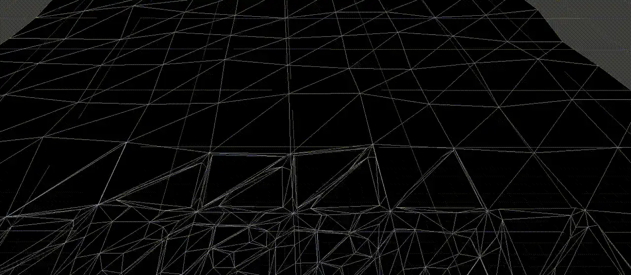
float4 GetTessellationFactors(float3 p1,float3 p2,float3 p3, ...){ float3 edgeFactors = float3( GetEdgeTessellationFactor(p1, p2, ...), GetEdgeTessellationFactor(p2, p3, ...), GetEdgeTessellationFactor(p3, p1, ...), ); return float4(edgeFactors, (edgeFactors.x + edgeFactors.y + edgeFactors.z) * 0.2); // Here dividing by 5 yielded a better scaling of the internal factor compared to just the average. }Here is the final tessellation result.
Limits and Next Steps
While we finally have all the elements for making a water material, the one we have made is far from perfect. Here is a list of limits and what can and will be improved on:
- The current model works well with Blinn-Phong shading, a bit less with PBR as we have no precise way of computing where the water should be rougher (i.e. foam). It still does yield a decent enough look with some authoring.
- The signal we generate obviously tiles over a long enough space (as it can be seen from the initial animation). There is no way around this problem and the only solution is to find an algorithm that doesn’t tile (e.g. FFT based simulation)
- The algorithm doesn’t perform too well when using big amplitudes, and is best used in the case of shallow sea waves and small bodies of water (ponds, puddles etc…)
- Since there is no actual phyisics simulation, the water will not react to the presence of an object in it, but this is a different kind of problem which can and should be solved separately as for any large body of water the impact with something like a rock will visually affect the water movement only locally. We can optimize the computation by having only the area around the object be collision aware.
Once again, all the code for this can be ultimately found here.
I hope that this might help someone understand the maths involved with procedural generation a little better, as well as showcase how rooting a process into mathematical forms allows us to leverage all kinds of properties, ultimately making our lives easier along the way.
As the next steps I do plan on delving into the more advanced algorithm for generating waves, FFT based Ocean simulation.